There are three commonly used environments in the math mode:
math environment: Used for
formulas in running text
displaymath environment:
Used to display longer formulas
equation environment:
Used for displaying equations for numbering and cross reference
math environment is used to typeset short formulas in
the running text. Such formulas are called in-line or in-text
formulas. You can use this environment in any of the following
forms:
\begin{math} . . . \end{math}
Thus, you could have a line of LaTeX source code like this:
A circle in the $x$--$y$--plane has equation \( x^2 + y^2 = 1
\)  ...
.
Since there is usually no problem with matching the begin and end of
the math environments, you'll most often see $ . . . $. It is
best to avoid using this environment for long formulas.
The displaymath environment is used to typeset longer
formulas. It is better to have long formulas or equations displayed,
that is, indented and with whitespace above and below.
You can use this environment in any of the following forms:
\begin{displaymath} . . . \end{displaymath}
\[ . . . \]
$$ . . . $$; however, this last is not recommend in LaTeX2e.
The standard usage here is \[ . . . \], and it is a good
idea to put the opening \[ and closing \]
on separate lines.
The equation environment can be used by typing
\begin{equation} . . . \end{equation}.
The equations are numbered by LaTeX during the actual processing of the source file,
so the number that LaTeX assigns to a given equation can change if we insert other
equations before it. Later on we will see how to create a label for an equation
so that we can refer to the equation in the paper
without having to know which number will be assigned to it during typesetting.
That makes it easy to change our document without having to change all the cross
references --- one extremely handy feature of LaTeX.
We now look at some easy formulas. It turns out that even the most complicated formula can be built up systematically in LaTeX from simpler pieces, so that it is not extremely difficult to type complicated formulas.
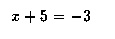
It is important to keep in mind that LaTeX has its own way of handling spacing in mathematics mode. It distinguishes between binary operators, like the + sign in the expression "3 + 5 = 8", and unary operators, like the - sign in the formula "x + 5 = -3". For example, consider the spacing of symbols in the typeset version of the formula
   \[
       x + 5 = -3
   \]
Here is how LaTeX typesets it.
If you want to typeset equations beyond the very simplest ones, you will want
to use the amsmath package, one of the many packages that you can
use with LaTeX. This package provides features for aligning several equations,
for handling multiline equations, compound symbols and certain kinds of diagrams.
The package is loaded into LaTeX by the command \usepackage{amsmath},
which goes in the preamble of the LaTeX source file (that is, between the
documentclass line and the begin{document} line).
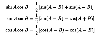
Here's an example of using the package to make some aligned equations.
   \documentclass[12pt]{article}
   \usepackage{amsmath}
       \begin{document}
          \begin{align*}
          \sin A \cos B &= \frac{1}{2}\left[ \sin(A-B)+\sin(A+B) \right] \\
          \sin A \sin B &= \frac{1}{2}\left[ \sin(A-B)-\cos(A+B) \right] \\
          \cos A \cos B &= \frac{1}{2}\left[ \cos(A-B)+\cos(A+B) \right] \\
          \end{align*}
       \end{document}
The align environment is a souped up version of the
equation environment. It uses the & symbol for
alignment, much like the tabular environment. The
align* version is the same as align except
that it doesn't produce equation numbers.
Here is how LaTeX typesets the above source file.
One can easily produce fractions, symbols for differentiation and integration, and so on. For example:
     \[
        \frac{d}{dx}\left( \int_{0}^{x} f(u)\,du\right)=f(x).
     \]
This typesets: 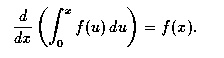
Moreover, if you know how to use the symbolic algebra package Maple V, you can get it to produce LaTeX code. The following LaTeX formula
\[
{\frac {d}{dx}}\arctan(\sin({x}^{2}))=-2\,{\frac {\cos({x}^{2})x}{-2+
\left (\cos({x}^{2})\right )^{2}}}
\]
is produced by the Maple V instruction:
latex(Diff(arctan(sin(x^2)),x)=simplify(diff(arctan(sin(x^2)),x)));
I just copied the output into this document by using the mouse, and added the lines \[ and \] for math mode.
Here is the typeset version:
